Integral Approximations

integral area

Integration is the best way to find the area from a curve to the axis, because we get a formula for an exact answer.

integral area small delta x

But when integration is hard (or impossible) we can instead add up lots of slices to get an approximate answer.

Let's have a go!

Examples

Let's use f(x) = ln(x) from x = 1 to x = 4

We actually can integrate that (this let's us check answers) and get the true answer of 2.54517744447956....

But imagine we can't, and all we can do is calculate values of ln(x):

at x=1: ln(1) = 0
at x=2: ln(2) = 0.693147...
etc

We will use a slice width of 1 to make it easy to see what is going on, but smaller slices are more accurate.

There are different methods we can use:

Left Rectangular Approximation Method (LRAM)

integral approximation Left Rectangular Graph

This method uses rectangles whose height is the left-most value. Areas are:

x=1 to 2: ln(1) × 1 = 0 × 1 = 0
x=2 to 3: ln(2) × 1 = 0.693147... × 1 = 0.693147...
x=3 to 4: ln(3) × 1 = 1.098612... × 1 = 1.098612...

Adding these up gets 1.791759, much lower than 2.545177. Why?

Because we are missing all that area between the tops of the rectangles and the curve.

This is made worse by a curve that is constantly increasing. When a curve goes up and down more, the error is usually less.

Right Rectangular Approximation Method (RRAM)

integral approximation Right Rectangular Graph

Here we calculate the rectangle's height using the right-most value. Areas are:

x=1 to 2: ln(2) × 1 = 0.693147... × 1 = 0.693147...
x=2 to 3: ln(3) × 1 = 1.098612... × 1 = 1.098612...
x=3 to 4: ln(4) × 1 = 1.386294... × 1 = 1.386294...

Adding these up gets 3.178054, which is now much higher than 2.545177, because of the extra areas between the tops of the rectangles and the curve.

Midpoint Rectangular Approximation Method (MRAM)

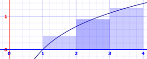
integral approximation Midpoint Rectangular Graph

We can also use the midpoint! Areas are:

x=1 to 2: ln(1.5) × 1 = 0.405465... × 1 = 0.405465...
x=2 to 3: ln(2.5) × 1 = 0.916291... × 1 = 0.916291...
x=3 to 4: ln(3.5) × 1 = 1.252763... × 1 = 1.252763...

Adding these up gets 2.574519..., which is quite close to 2.545177.

Trapezoidal Rule

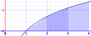
integral approximation: Trapezoidal Rule

We can have a sloped top! Each slice is now a trapezoid (or possibly a triangle), so it is called the Trapezoidal Rule.

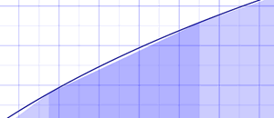
integral approximation: Trapezoidal Rule zoomed in

The calculation just averages the left and right values. Areas are:

x=1 to 2: ln(1) + ln(2) 2 × 1 = 0 + 0.693147...2 × 1 = 0.346573...
x=2 to 3: ln(2) + ln(3)2 × 1 = 0.693147... + 1.098612...2 × 1 = 0.895879...
x=3 to 4: ln(3) + ln(4)2 × 1 = 1.098612... + 1.386294...2 × 1 = 1.242453...

Adding these up gets 2.484907, which is still a bit lower than 2.545177, mostly because the curve is concave down over the interval.

Notice that in practice each value gets used twice (except first and last) and then the whole sum is divided by 2:

ln(1) + ln(2) 2 × 1 + ln(2) + ln(3) 2 × 1 + ln(3) + ln(4) 2 × 1

1 2 × ( ln(1) + ln(2) + ln(2) + ln(3) + ln(3) + ln(4) )

1 2 × ( ln(1) + 2 ln(2) + 2 ln(3) + ln(4) )

So we can have a general formula:

Δx 2 × ( f(x₀) + 2f(x₁) + 2f(x₂) + ... 2f(x_n−1) + f(x_n) )

By the way, this method is just the average of the Left and Right Methods:

Trapezoidal Approximation = LRAM + RRAM 2

Note: the previous 4 methods are also called Riemann Sums after the mathematician Bernhard Riemann.

Simpson's Rule

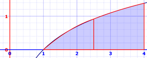
integral approximation: Simpsons Rule

An improvement on the Trapezoidal Rule is Simpson's Rule. It is based on using parabolas at the top instead of straight lines. The parabolas often get quite close to the real curve:

integral approximation: Simpsons Rule zoomed in

It sounds hard, but we end up with a formula like the trapezoid formula, but we divide by 3 and use a 1, 4, 2, ..., 2, 4, 1 pattern of factors:

Δx 3 × ( f(x₀) + 4f(x₁) + 2f(x₂) + ... 4f(x_n−1) + f(x_n) )

But: n must be even. So let's take 6 slices of 0.5 each:

0.5 3 × ( f(1) + 4f(1.5) + 2f(2) + 4f(2.5) + 2f(3) + 4f(3.5) + f(4) )

Plugging in values of ln(1) etc gives:

0.5 3 × ( 15.2679... )

2.544648...

This is a great result when compared to 2.545177....

Plus and Minus

definite integral cos(x) from 1 to 3

When the curve is below the axis the value of the integral is negative!

So we get a "net" value.

If we want a total area (say we wanted to paint it) we can use the absolute value function abs(). Or manually find where the curve crosses the axis and then work out separate integrals and reverse the negatives before adding.

Error and Accuracy

Let's compare them all:

f(x)=ln(x)	N = 3		N = 6		N = 100
	Estimation	Error	Estimation	Error	Estimation	Error
LRAM	1.791759	0.753418	2.183140	0.362037	2.524327	0.020850
RRAM	3.178054	-0.632877	2.876287	-0.331110	2.565916	-0.020739
MRAM	2.574519	-0.029342	2.552851	-0.007674	2.545206	-0.000029
Trapezoidal Rule	2.484907	0.060271	2.529713	0.015464	2.545121	0.000055
Simpson’s Rule	(N must be even)		2.544648	0.000529	2.545177	<0.000001

Simpson’s Rule rules! And it is just as easy to use as the others.

Of course a different function will produce different results. Why not try some yourself?

Maximum Error

Often we won't know the actual answer ... so how do we know how good our estimate is?

You can get a good feel by trying different slice widths.

And there are also these formulas for the maximum error of approximation (these are for the worst case and the actual error will hopefully be a lot smaller):

For Midpoint: |E| = K(b-a)³ 24n²

For Trapezoidal: |E| = K(b-a)³ 12n²

For Simpson's: |E| = M(b-a)⁵ 180n⁴

Where:

|E| is the absolute value of the maximum error (could be plus or minus)
a is the start of the interval
b is the end of the interval
n is the number of slices
K is the greatest second derivative over the interval.
M is the greatest fourth derivative over the interval.

(By "greatest" we mean the maximum absolute value.)

a, b and n are easy, but how do we find K and M ?

Example: f(x) = ln(x) between 1 and 4

Let's find some derivatives first, we will need them:

1^st derivative: f'(x) = 1/x
2^nd derivative: f''(x) = −1/x²
3^rd derivative: f⁽³⁾(x) = 2/x³
4^th derivative: f⁽⁴⁾(x) = −6/x⁴
5^th derivative: f⁽⁵⁾(x) = 24/x⁵

The greatest K could be at the start, end, or somewhere in between:

Start: f''(1) = −1/1² = −1
End: f''(4) = −1/4² = −1/16
In between: use the 3^rd derivative to see if there are zeros in the 1 to 4 interval, which could mean a change in direction.
Does f⁽³⁾(x) = 0 between 1 and 4? No. So the maximum is at start or end.

So K = 1 (the maximum absolute value)

Same for M, but higher derivatives:

Start: f⁽⁴⁾(1) = −6/1⁴ = −6
End: f⁽⁴⁾(4) = −6/4⁴= −6/256
In between: use the 5^th derivative to see if there are zeros in the 1 to 4 interval.
Does f⁽⁵⁾(x) = 24/x⁵ equal zero between 1 and 4? No.

So M = 6 (the maximum absolute value)

For just 6 slices, the Maximum Errors are:

Midpoint: |E| = 1(4−1)³ 24×6² = 0.03125

Trapezoidal: |E| = 1(4−1)³ 12×6² = 0.0625

Simpson's: |E| = 6(4−1)⁵ 180×6⁴ = 0.00625

Shapes we Know

The curve may have a shape we know, and we can use geometry formulas like these examples:

Example: Triangle

integral approximation triangle
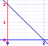
f(x) = 2 − x, from 0 to 2

A = ½ × 2 × 2 = 2

Example: Rectangle

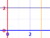
integral approximation rectangle
f(x) = 2, from 0 to 3

A = 2 × 3 = 6

Example: Semicircle

integral approximation circle
f(x) = √(1 − x²), from −1 to +1

A = π r² / 2 = π / 2

Conclusion

We can estimate the area under a curve by slicing a function up

There are many ways of finding the area of each slice such as:

Left Rectangular Approximation Method (LRAM)
Right Rectangular Approximation Method (RRAM)
Midpoint Rectangular Approximation Method (MRAM)
Trapezoidal Rule
Simpson's Rule

We can use error formulas to find the largest possible error in our estimate

Basic geometry formulas can sometimes help us find areas under the curve